Students can download 12th Business Maths Chapter 6 Random Variable and Mathematical Expectation Ex 6.1 Questions and Answers, Samacheer Kalvi 12th Business Maths Book Solutions Guide Pdf helps you to revise the complete Tamilnadu State Board New Syllabus and score more marks in your examinations.
Tamilnadu Samacheer Kalvi 12th Business Maths Solutions Chapter 6 Random Variable and Mathematical Expectation Ex 6.1
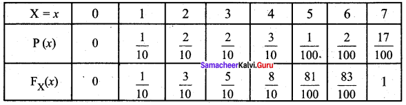
Question 1.
Construct cumulative distribution function for the given probability distribution.
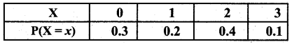
Solution:
Thus the cumulative distribution function is given by,
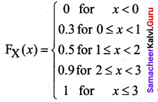
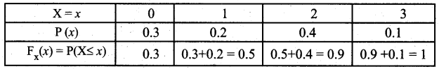
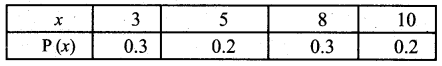
Question 2.
Let X be a discrete random variable with the following p.m.f.
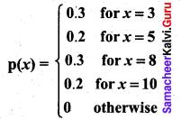
Find and plot the c.d.f. of X.
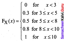
Solution:
The probability distribution function can be written as follows:
We obtain
F(3) = P(x ≤ 3) = P(3) = 0.3
F(5) = P(x ≤ 5) = P(3) + P(5) = 0.3 + 0.2 = 0.5
F(8) = P(x ≤ 8) = P(3) + P(5) + P(8) = 0.5 + 0.3 = 0.8
F(10) = P(x ≤ 10) = P(3) + P(5) + P(8) + P(10) = 0.8 + 0.2 = 1
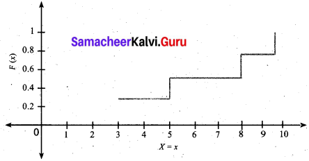
![]()
Question 3.
The discrete random variable X has the following probability function.
where k is a constant. Show that k = \(\frac{1}{18}\)
Solution:
The given probability function can be written as follows:
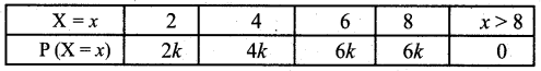
Since the condition of probability mass function is \(\sum_{i=1}^{\infty} p\left(x_{i}\right)=1\), we have
2k + 4k + 6k + 6k = 1
⇒ 18k = 1
⇒ k = \(\frac{1}{18}\)
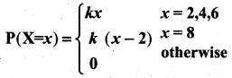
Question 4.
The discrete random variable X has the probability function.
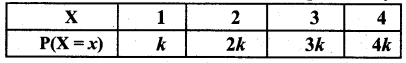
Show that k = 0.1
Solution:
From the data
P(x = 1) = k
p(x = 2) = 2k
p(x = 3) = 3k
P(x = 4) = 4k
Since P(X = x) is a probability Mass function
\(\sum_{x=1}^{4}\) P(X = x) = 1
\(\sum_{i=1}^{∞}\) P(xi) = 1
p(x = 1) + P(x = 2) + P(x = 3) + P(x = 4) = 1
P(x = 1) + P(x = = 2) + P(x = 3) + P(x = 4) = 1
k + 2k + 3k + 4k = 1
10k = 1
k = \(\frac { 1 }{10}\)
∴ k = 0.1
![]()
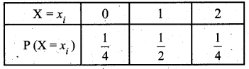
Question 5.
Two coins are tossed simultaneously. Getting a head is termed a success. Find the probability distribution of the number of successes.
Solution:
Let X be the number of observed heads. The sample space S = {(H H), (H T), (T H), (T T)}
X takes the values 2, 1, 1, 0. Hence the probability distribution of the number of successes is given by
Question 6.
A random variable X has the following probability function.

(i) Find k
(ii) Evaluate P( X < 6), P(X ≥ 6) and P(0 < X < 5)
(iii) If P(X ≤ x) > \(\frac{1}{2}\), then find the minimum value of x.
Solution:
(i) Since the condition of Probability Mass function
\(\sum_{i=2}^{∞}\) P(xi) = 1
\(\sum_{i=0}^{7}\) P(xi) = 1
P(x = 0) + P(x = 1) + P(x = 2) + P(x = 3) + P(x = 4) + P P(x = 6) + p(x = 7) = 1
0 + k + 2k + 2k + 3k + k² + 2k² + 7k² + k = 1
10k² + 9k – 1 = 0
10k² + 10k – k – 1 = 0
10k(k + 1) -1(k + 1) = 0
(k + 1)(10k – 1) = 0
k + 1 = 0; 10k – 1 = 0
k = -1 10k = 1
k = \(\frac { 1 }{10}\)
k = -1 is not possible
![]()
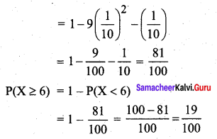
(ii) P(X < 6) = P(X = 0) + P(X = 1) + P(X = 2) + P (X = 3) + P(X = 4) + P (X = 5)
= 0 + k + 2k + 2k + 3k + k2
= 8k + k2
= 8(\(\frac{1}{10}\)) + (\(\frac{1}{10}\))2 (∵ k = \(\frac{1}{10}\))
= \(\frac{8}{10}+\frac{1}{100}=\frac{81}{100}\)
Method 2:
P(X < 6) = 1 – P(X ≥ 6)
= 1 – [P(X = 6) + P (X = 7)]
= 1 – [2k2 + 7k2 + k]
= 1 – 9k2 – k
P(0 < X < 5) = P(X = 1) + P(X = 2) + P (X = 3) + P(X = 4)
= k + 2k + 2k + 3k = 8k
= \(\frac{8}{10}\)
(iii) P(X ≤ x) > \(\frac{1}{2}\)
To find the minimum value of x, let us construct the cumulative distribution function of X.
From the table, we see that
P(X ≤ 0) = 0
P(X ≤ 1) = \(\frac{1}{10}\) = 0.1
P(X ≤ 2) = \(\frac{3}{10}\) = 0.3
P(X ≤ 3) = \(\frac{5}{10}\) = 0.5
P(X ≤ 4) = \(\frac{8}{10}\) = 0.8
So x = 4
![]()
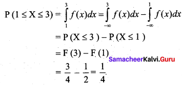
Question 7.
The distribution of a continuous random variable X in range (-3, 3) is given by p.d.f.
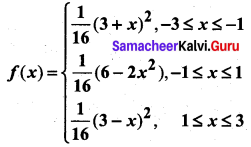
Verify that the area under the curve is unity.
Solution:
We know that area under a curve f(x) between x = a and x = b is \(\int_{a}^{b} f(x) d x\)
Here the area is given by \(\int_{-3}^{3} f(x) d x\)
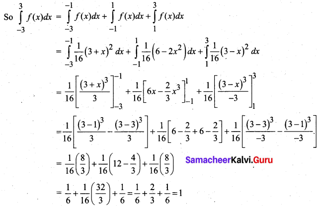
Thus the area under the curve is unity.
Question 8.
A continuous random variable X has the following distribution function:
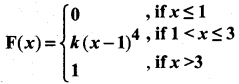
Find (i) k and (ii) the probability density function.
Solution:
(i) Here F(3) – F(1) = 1
K(3 – 1)4 – O = 1
K(2)4 = 1
K(16) = 1
k = \(\frac { 1 }{16}\)
(ii) The Probability density function
f(x) = \(\frac { d(F(x)) }{dx}\) = \(\left\{\begin{array}{l}
4 k(x-1)^{3}, 1<x \leq 3 \\
0 \text { else where }
\end{array}\right.\)
![]()
Question 9.
The length of time (in minutes) that a certain person speaks on the telephone is found to be a random phenomenon, with a probability function specified by the probability density function f(x) as
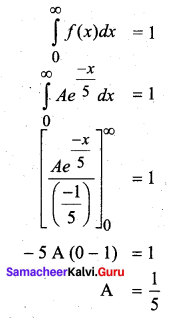
(a) Find the value of A that makes f(x) a p.d.f.
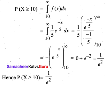
(b) What is the probability that the number of minutes that person will talk over the phone is (i) more than 10 minutes, (ii) less than 5 minutes and (iii) between 5 and 10 minutes.
Solution:
(a) For f(x) to be a p.d.f we must have \(\int_{-\infty}^{\infty} f(x) d x=1\)
According to the problem,
(b) (i) The probability that the number of minutes that person will talk is more than 10 minutes is given by
(b) (ii) The probability that the number of minutes is less than 5 is given by 5
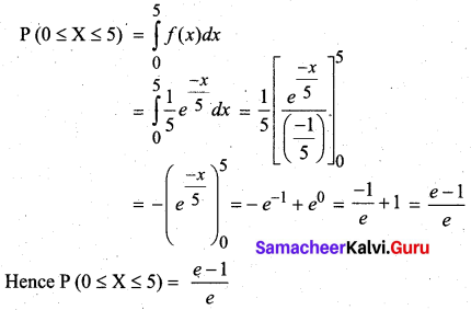
(b) (iii) The probability that the number of minutes that person will talk is between 5 and 10 minutes is given by
Question 10.
Suppose that the time in minutes that a person has to wait at a certain station for a train is found to be a random phenomenon with a probability function specified by the distribution function.
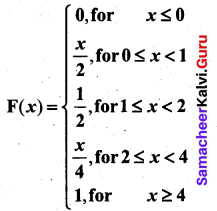
(a) Is the distribution function continuous? If so, give its probability density function?
(b) What is the probability that a person will have to wait (i) more than 3 minutes, (ii) less than 3 minutes and (iii) between 1 and 3 minutes?
Solution:
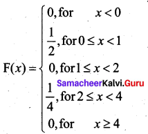
(a) Yes. The distribution function is continuous. It is defined for all values of -∞ < x < ∞.
We know that \(\frac{d}{d x}\) F(x) = f(x). So we differentiate the given distribution function in the intervals where it is defined to find the density function.
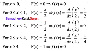
Thus the probability density function is given by
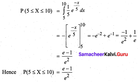
(b) (i) The probability that a person will have to wait for more than 3 minutes is given by
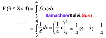
Method 2:
P (X ≥ 3) = 1 – P(X ≤ 3) = 1 – F(3)
From the question F (3) = \(\frac{3}{4}\)
So P (X ≥ 3) = 1 – \(\frac{3}{4}\) = \(\frac{1}{4}\)
(b) (ii) The probability that a person will have to Wait for less than 3 minutes is
P(X ≤ 3) = F(3) = \(\frac{3}{4}\)
(b) (iii) Probability that the person will have to wait between 1 and 3 minutes is
![]()
Question 11.
Define the random variable.
Solution:
A random variable (r.v.) is a real-valued function defined on a sample space S and taking values in (-∞, ∞) or whose possible values are numerical outcomes of a random experiment.
Question 12.
Explain what are the types of a random variable?
Solution:
Random variables are classified into two types namely discrete and continuous random variables.
Discrete random variable: A discrete random variable has a finite number of possible values or an infinite sequence of countable real numbers.
Examples:
- X denotes the number of hits when trying 20 free throws.
- X denotes the number of customers who arrive at the bank from 8.30 – 9.30 AM Mon – Fri.
- X denotes the number of balls sold during a week in a particular shop.
Continuous random variable:
A continuous random variable takes all values in an interval of real numbers.
Examples:
- X denotes the time it takes for a bulb to bum out.
- X denotes the weight of a truck in a truck – weighing station.
- X denotes the amount of water in a bottle.
![]()
Question 13.
Define discrete random variables.
Solution:
A variable which can assume a finite number of possible values or an infinite sequence of countable real numbers is called a discrete random variable.
Question 14.
What do you understand by continuous random variables?
Solution:
A random variable which can take on any value (integral as well as fraction) in the interval is called a continuous random variable.
Examples:
- The speed of a train.
- Electricity consumption in kilowatt-hours.
- Height of people in a population
- Weight of students in a class.
![]()
Question 15.
Describe what is meant by a random variable.
Solution:
If S is a sample space with a probability measure and x is a real-valued function defined over the elements of S then x is called a random variable A random variable is also called a change variable.
Question 16.
Distinguish between discrete and continuous random variables.
Solution:
| Discrete Variable | Continuous Variable |
| 1. A variable which can take only certain values. | 1. A variable which can take any value in a particular limit. |
| 2. The value of the variables can increase incomplete numbers. | 2. Its value increases infractions but not in jumps. |
| 3. Example: Number of students who opt for commerce in class 11, say 30, 35, 40, 45, and 50. | 3. Example: Height, Weight and age of family members: 50.5 kg, 30 kg, 42.8 kg and 18.6 kg. |
| 4. Binomial, Poisson, Hypergeometric probability distributions come under this category. | 4. Normal, student’s t and chi-square distribution come under this category. |
Question 17.
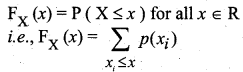
Explain the distribution function of a random variable.
Solution:
The discrete cumulative distribution function or distribution function of a real-valued discrete random variable X, which takes the countable number of points x1, x2,….. with corresponding probabilities p(x1), p(x2),…. is defined by
If X is a continuous random variable with probability density function fx(x), then the function FX(x) is defined by
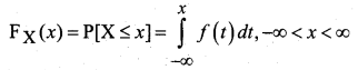
is called the distribution function of the continuous random variable.
![]()
Question 18.
Explain the terms
(i) Probability mass function
(ii) Probability density function and
(iii) Probability distribution function.
Solution:
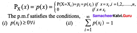
(i) Probability mass function: A probability mass function (p.m.f) is a function that gives the probability that a discrete random variable is exactly equal to some value. This is the means of defining a discrete probability distribution. Let X be a random variable with values x1, x2,…. xn….. Then the p.m.f is defined by
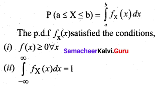
(ii) Probability density function: A probability density function (p.d.f) or density of a continuous random variable, is a function whose value at any given sample (or point) in the sample space gives the probability of the r.v. falling within the range of values. This probability is given by the area under the density function. The probability that an r.v. X takes a value in the interval [a, b] is given by
(iii) Probability distribution function: A probability distribution is a list of all of the possible outcomes of a random variable along with their corresponding probability values. When the r.v is discrete, the distribution function is called a probability mass function (p.m.f), and when the r.v is continuous, the distribution function is called a probability density function (p.d.f)
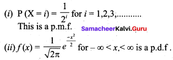
Examples:
Question 19.
What are the properties of
(i) discrete random variable and
(ii) continuous random variable?
Solution:
(i) The probability mass function p(x) must satisfy the following conditions
- p(xi) ≥ 0 ∀ i,
- \(\sum_{i=1}^{∞}\) p(xi) = 1
(ii) The probability density functions/)(x) or simply ; by/(x) must satisfy the following conditions.
- f(x) ≥ 0 ∀ x and
- \(\int_{-∞}^{∞}\) f(x) dx = 1
![]()
Question 20.
State the properties of the distribution function.
Solution:
The function Fx(x) or simply F(x) has the following properties.
(i) 0 ≤ F(x) ≤ 1, -∞ < x < ∞
(ii) F(-∞) = \(\lim _{x \rightarrow-\infty}\) F(x) = 0 and F(+∞) = \(\lim _{x \rightarrow ∞}\) F(x) = 1.
(iii) F(.) is a monotone, non-decreasing function; ; that is, F(a) < F(b) for a < b.
(iv)F(.) is continuous from the right; that is, \(\lim _{h \rightarrow 0}\) F(x + h) = F(x).
(v) F(x) = \(\frac { d }{dx}\) F(x) = f(x) ≥ 0;
(vi) F'(x) = \(\frac { d }{dx}\) F(x) = f(x) ⇒ dF(x) = f(x)dx
dF(x) is known as probability differential of X.
(vii) P(a ≤ x ≤ b) = \(\int_{a}^{b}\) f(x)dx = \(\int_{-∞}^{b}\) f(x)dx – \(\int_{-∞}^{a}\) f(x)dx
= P(X ≤ b) – P(X ≤ a)
= F(b) – F(a)